The pytesmo validation framework
The pytesmo validation framework takes care of iterating over datasets, spatial and temporal matching as well as scaling. It uses metric calculators to then calculate metrics that are returned to the user. There are several metrics calculators included in pytesmo but new ones can be added simply.
Overview
How does the validation framework work? It makes these assumptions about the used datasets:
The dataset readers that are used have a method for reading data (usually called
read) that can be called either by a grid point index (gpi) which can be any indicator that identifies a certain grid point or by using longitude and latitude. This means that both call signaturesread(gpi)andread(lon, lat)must be valid. Please check the pygeobase documentation for more details on how a fully compatible dataset class should look. But a simplereadmethod should do for the validation framework. This assumption can be relaxed by using theread_ts_nameskeyword in the pytesmo.validation_framework.data_manager.DataManager class.The reading method returns a pandas.DataFrame time series.
Ideally the datasets classes also have a
gridattribute that is a pygeogrids grid. This makes the calculation of lookup tables easily possible and the nearest neighbor search faster.
Fortunately these assumptions are true about the dataset readers included in pytesmo.
It also makes a few assumptions about how to perform a validation. For a comparison study it is often necessary to choose a spatial reference grid, a temporal reference and a scaling or data space reference.
Spatial reference
The spatial reference is the one to which all the other datasets are matched spatially. Often through nearest neighbor search. The validation framework uses grid points of the dataset specified as the spatial reference to spatially match all the other datasets with nearest neighbor search. Other, more sophisticated spatial matching algorithms are not implemented at the moment. If you need a more complex spatial matching then a preprocessing of the data is the only option at the moment.
Temporal reference
The temporal reference is the dataset to which the other dataset are temporally matched. That means that the nearest observation to the reference timestamps in a certain time window is chosen for each comparison dataset. This is by default done by the temporal matching module included in pytesmo. How many datasets should be matched to the reference dataset at once can be configured, we will cover how to do this later.
Data space reference
It is often necessary to bring all the datasets into a common data space by using. Scaling is often used for that and pytesmo offers a choice of several scaling algorithms (e.g. CDF matching, min-max scaling, mean-std scaling, triple collocation based scaling). The data space reference can also be chosen independently from the other two references.
Data Flow
After it is initialized, the validation framework works through the following steps:
Read all the datasets for a certain job (gpi, lon, lat)
Read all the masking dataset if any
Mask the temporal reference dataset using the masking data
Temporally match all the chosen combinations of temporal reference and other datasets
Turn the temporally matched time series over to the metric calculators
Get the calculated metrics from the metric calculators
Put all the metrics into a dictionary by dataset combination and return them.
Masking datasets
Masking datasets can be used if the datasets that are compared do not contain the necessary information to mask them. For example we might want to use modelled soil temperature data to mask our soil moisture observations before comparing them. To be able to do that we just need a Dataset that returns a pandas.DataFrame with one column of boolean data type. Everywhere where the masking dataset is True the data will be masked.
Let’s look at a first example.
Example soil moisture validation: ASCAT - ISMN
This example shows how to setup the pytesmo validation framework to perform a comparison between ASCAT and ISMN data.
[ ]:
import os
import numpy as np
from pathlib import Path
from pprint import pprint
import pytesmo.validation_framework.metric_calculators as metrics_calculators
from datetime import datetime
import warnings
from ascat.read_native.cdr import AscatGriddedNcTs

from ismn.interface import ISMN_Interface  # install ismn: 'pip install ismn'
from pytesmo.validation_framework.validation import Validation
from pytesmo.validation_framework.results_manager import netcdf_results_manager
from pytesmo.utils import rootdir

import tempfile
You need the test data from https://github.com/TUW-GEO/pytesmo-test-data for this example
[2]:
from tempfile import mkdtemp
output_folder = Path(mkdtemp())
print('Data is stored in:', output_folder)
Data is stored in: /tmp/tmppeisd__e
First we initialize the data readers that we want to use. In this case the ASCAT soil moisture time series and in situ data from the ISMN.
Initialize ASCAT reader
[3]:
testdata_path = rootdir() / "tests" / "test-data"
ascat_data_folder = testdata_path / "sat" / "ascat" / "netcdf" / "55R22"
ascat_grid_fname = testdata_path / "sat" / "ascat" / "netcdf" / "grid" / "TUW_WARP5_grid_info_2_1.nc"
static_layer_path = testdata_path / "sat" / "h_saf" / "static_layer"


#init the AscatSsmCdr reader with the paths
with warnings.catch_warnings():
    warnings.filterwarnings('ignore') # some warnings are expected and ignored

    ascat_reader = AscatGriddedNcTs(
        ascat_data_folder,
        "TUW_METOP_ASCAT_WARP55R22_{:04d}",
        grid_filename=ascat_grid_fname,
        static_layer_path=static_layer_path
    )

ascat_reader.read_bulk = True
Initialize ISMN reader
[4]:
ismn_data_folder = testdata_path / "ismn/multinetwork/header_values"
meta_path = tempfile.mkdtemp()
ismn_reader = ISMN_Interface(ismn_data_folder, meta_path=meta_path)
Processing metadata for all ismn stations into folder /home/wpreimes/shares/home/code/pytesmo/tests/test-data/ismn/multinetwork/header_values.
This may take a few minutes, but is only done once...
Hint: Use `parallel=True` to speed up metadata generation for large datasets
Files Processed: 100%|██████████| 8/8 [00:00<00:00, 65.44it/s]
Metadata generation finished after 0 Seconds.
Metadata and Log stored in /tmp/tmp_72gspsz
Found existing ismn metadata in /tmp/tmp_72gspsz/header_values.csv.
The validation is run based on jobs. A job consists of at least three lists or numpy arrays specifing the grid point index, its latitude and longitude. In the case of the ISMN we can use the dataset_ids that identify every time series in the downloaded ISMN data as our grid point index. We can then get longitude and latitude from the metadata of the dataset.
DO NOT CHANGE the name jobs because it will be searched during the parallel processing!
[5]:
jobs = []

ids = ismn_reader.get_dataset_ids(variable='soil_moisture', min_depth=0, max_depth=0.1)

for idx in ids:
    metadata = ismn_reader.read_metadata(idx)
    jobs.append((idx, metadata['longitude'].val, metadata['latitude'].val))
    break

print("Jobs (gpi, lon, lat):")
print(jobs)
Jobs (gpi, lon, lat):
[(0, 102.1333, 33.8833)]
For this example we only process one job / pixel / sensor.
It is important here that the ISMN reader has a reading function that works by just using the dataset_id. In this way the validation framework can go through the jobs and read the correct time series.
[6]:
data = ismn_reader.read(ids[0])
print('ISMN data example:')
print(data.head())
ISMN data example:
                     soil_moisture soil_moisture_flag soil_moisture_orig_flag
date_time
2008-07-01 00:00:00            0.5                C03                       M
2008-07-01 01:00:00            0.5                C03                       M
2008-07-01 02:00:00            0.5                C03                       M
2008-07-01 03:00:00            0.5                C03                       M
2008-07-01 04:00:00            0.5                C03                       M
Initialize the Validation class
The Validation class is the heart of the validation framework. It contains the information about which datasets to read using which arguments or keywords and if they are spatially compatible. It also contains the settings about which metric calculators to use and how to perform the scaling into the reference data space. It is initialized in the following way:
[7]:
datasets = {
    'ISMN': {
        'class': ismn_reader,
        'columns': ['soil_moisture']
    },
    'ASCAT': {
        'class': ascat_reader,
        'columns': ['sm'],
        'kwargs': {'mask_frozen_prob': 80,
                   'mask_snow_prob': 80,
                   'mask_ssf': True}
    }}
The datasets dictionary contains all the information about the datasets to read. The class is the dataset class to use which we have already initialized. The columns key describes which columns of the dataset interest us for validation. This a mandatory field telling the framework which other columns to ignore. In this case the columns soil moisture_flag and soil moisture_orig_flag will be ignored by the ISMN reader. We can also specify additional keywords that should be given to
the read method of the dataset reader. In this case we want the ASCAT reader to mask the ASCAT soil moisture using the included frozen and snow probabilities as well as the SSF. There are also other keys that can be used here. Please see the documentation for explanations.
[10]:
period = [datetime(2007, 1, 1), datetime(2014, 12, 31)]
basic_metrics = metrics_calculators.PairwiseIntercomparisonMetrics()

process = Validation(
    datasets, 'ISMN',
    temporal_ref='ASCAT',
    scaling='mean_std',
    scaling_ref='ASCAT',
    metrics_calculators={(2, 2): basic_metrics.calc_metrics},
    period=period)
/home/wpreimes/shares/home/code/pytesmo/src/pytesmo/validation_framework/validation.py:144: UserWarning: You are using the default temporal matcher. If you are using one of the newer metric calculators (PairwiseIntercomparisonMetrics, TripleCollocationMetrics) you should probably use `make_combined_temporal_matcher` instead. Have a look at the documentation of the metric calculators for more info.
  warnings.warn(
During the initialization of the Validation class we can also tell it other things that it needs to know. In this case it uses the datasets we have specified earlier. The spatial reference is the 'ISMN' dataset which is the second argument. The ‘metrics_calculators’ argument looks a little bit strange so let’s look at it in more detail.
It is a dictionary with a tuple as the key and a function as the value. The key tuple (n, k) has the following meaning: n datasets are temporally matched together and then given in sets of k columns to the metric calculator. The metric calculator then gets a DataFrame with the columns [‘ref’, ‘k1’, ‘k2’ …] and so on depending on the value of k. The value of (2, 2) makes sense here since we only have two datasets and all our metrics also take two inputs.
This can be used in more complex scenarios to e.g. have three input datasets that are all temporally matched together and then combinations of two input datasets are given to one metric calculator while all three datasets are given to another metric calculator. This could look like this:
{ (3 ,2): metric_calc,
  (3, 3): triple_collocation}
Create the variable save_path which is a string representing the path where the results will be saved. DO NOT CHANGE the name save_path because it will be searched during the parallel processing!
[11]:
save_path = output_folder / 'ascat_ismn'

for job in jobs:

    results = process.calc(*job)
    pprint(results)
    netcdf_results_manager(results, save_path)
{(('ASCAT', 'sm'), ('ISMN', 'soil_moisture')): {'BIAS': array([1.4210855e-14], dtype=float32),
                                                'BIAS_ci_lower': array([-1.124606], dtype=float32),
                                                'BIAS_ci_upper': array([1.124606], dtype=float32),
                                                'R': array([0.5342869], dtype=float32),
                                                'RMSD': array([10.789426], dtype=float32),
                                                'RSS': array([41558.98], dtype=float32),
                                                'R_ci_lower': array([0.45576647], dtype=float32),
                                                'R_ci_upper': array([0.60455596], dtype=float32),
                                                'gpi': array([0], dtype=int32),
                                                'lat': array([33.8833]),
                                                'lon': array([102.1333]),
                                                'mse': array([116.41171], dtype=float32),
                                                'mse_bias': array([2.019484e-28], dtype=float32),
                                                'mse_corr': array([116.41171], dtype=float32),
                                                'mse_var': array([3.1554436e-30], dtype=float32),
                                                'n_obs': array([357], dtype=int32),
                                                'p_R': array([9.664754e-28], dtype=float32),
                                                'p_rho': array([2.471651e-28], dtype=float32),
                                                'p_tau': array([2.1020434e-26], dtype=float32),
                                                'rho': array([0.53934574], dtype=float32),
                                                'rho_ci_lower': array([0.45559874], dtype=float32),
                                                'rho_ci_upper': array([0.61362934], dtype=float32),
                                                'status': array([0], dtype=int32),
                                                'tau': array([0.3907124], dtype=float32),
                                                'tau_ci_lower': array([0.35201582], dtype=float32),
                                                'tau_ci_upper': array([0.42807564], dtype=float32),
                                                'urmsd': array([10.789426], dtype=float32),
                                                'urmsd_ci_lower': array([10.065898], dtype=float32),
                                                'urmsd_ci_upper': array([11.661137], dtype=float32)}}
The validation is then performed by looping over all the defined jobs and storing the results. You can see that the results are a dictionary where the key is a tuple defining the exact combination of datasets and columns that were used for the calculation of the metrics. The metrics itself are a dictionary of metric-name: numpy.ndarray which also include information about the gpi, lon and lat. Since all the information contained in the job is given to the metric calculator they can be
stored in the results.
Storing of the results to disk is at the moment supported by the netcdf_results_manager which creates a netCDF file for each dataset combination and stores each metric as a variable. We can inspect the stored netCDF file which is named after the dictionary key:
[12]:
import netCDF4
results_fname = Path(save_path) / "ASCAT.sm_with_ISMN.soil_moisture.nc"

with netCDF4.Dataset(str(results_fname)) as ds:
    for var in ds.variables:
        print(var, ds.variables[var][:])
lon [102.1333]
lat [33.8833]
idx [0]
_row_size [0]
time []
gpi [0]
status [0]
R [0.5342869]
p_R [9.664754e-28]
BIAS [1.4210855e-14]
RMSD [10.789426]
mse [116.41171]
RSS [41558.98]
mse_corr [116.41171]
mse_bias [2.019484e-28]
urmsd [10.789426]
mse_var [3.1554436e-30]
rho [0.53934574]
p_rho [2.471651e-28]
tau [0.3907124]
p_tau [2.1020434e-26]
BIAS_ci_lower [-1.124606]
BIAS_ci_upper [1.124606]
urmsd_ci_lower [10.065898]
urmsd_ci_upper [11.661137]
R_ci_lower [0.45576647]
R_ci_upper [0.60455596]
rho_ci_lower [0.45559874]
rho_ci_upper [0.61362934]
tau_ci_lower [0.35201582]
tau_ci_upper [0.42807564]
n_obs [357]
Metric Calculator Adapters
Metric calculators compute a set of comparison metrics based on the passed input. Usually the input are two or more collocated time series. However, to validate soil moisture it is often desired to assess the quality for certain temporal subsets independently. E.g. if a varying level of agreement between two datasets is expected for two different seasons (e.g. wet/dry season, summer/winter) or if the varying level of agreement should be assessed (e.g. on a seasonal/monthly basis). In this case
pytesmo provides adapters to split up the input time series before computing validation metrics. These adapters work with any (properly implemented) metric calculator. You can use one of the predefined adapters in pytesmo.validation_framework.metric_calculators_adapters. Currently, there are 2 options:
SubsetsMetricsAdapter: This adapter lets you define arbitrary temporal subsets of your time series data before metrics computation. You can compute metrics for a certain set of datetimes or datetime ranges.MonthsMetricsAdapter: This is a version of a SubsetsMetricsAdapter that allows splitting up the data based on their month. You can e.g. compute validation metrics for each month of a year individually, or for each season (i.e. 3 * 4 months), or any other combination of months.
Let’s look at an example. Here we use the base SubsetsMetricsAdapter. We compute the same metrics as before, but apply the metrics calculator to a set of predefined temporal subgroups. Note that groups in this example were chosen to demonstrate the feature range of the TsDistributor rather than to produce meaningful results.
We create a SubsetsMetricsAdapter that takes the original metrics calculator and a list of named, temporal subsets (dict).
[13]:
import os
from pytesmo.validation_framework.metric_calculators_adapters import SubsetsMetricsAdapter, TsDistributor
from pytesmo.time_series.grouping import YearlessDatetime
from datetime import datetime
import shutil

subsets = {
    # The first subset does only include values in August 2010 and 2011 + July 31st of both years
    'August2010/11': TsDistributor(dates=[datetime(year=2009, month=7, day=31), datetime(2010, 7, 31)],
                                   date_ranges=[(datetime(2010, 7, 1, 0, 0), datetime(2010, 7, 31)),
                                                (datetime(2011, 7, 1), datetime(2011, 7, 31))]),

    # The second subset includes all values from June to September of ANY YEAR, but not August
    'JJS': TsDistributor(yearless_date_ranges=[
        (YearlessDatetime(month=6, day=1, hour=0, minute=0), YearlessDatetime(7, 31)),
        (YearlessDatetime(9, 1), YearlessDatetime(9, 30))
    ]),

    # The third group includes all values from Feb 28th to the end of April of ANY YEAR
    'MarchApril': TsDistributor(yearless_date_ranges=[(YearlessDatetime(2, 28), YearlessDatetime(4, 30))]),
}

adapted_intercomparison_metrics = SubsetsMetricsAdapter(
    metrics_calculators.PairwiseIntercomparisonMetrics(calc_kendall=False, calc_spearman=False),
    subsets,
    group_results='join')
The adapted metrics calculator can now be used as before. The results will contain the chosen group names accordingly, as defined in the adapter. The results manager will write them to a netcdf file. Note that this only works as group_results='join' was selected, otherwise the output format would different from what the results manager expects.
[14]:
import pandas as pd
from pytesmo.validation_framework.temporal_matchers import make_combined_temporal_matcher
process = Validation(
    datasets, 'ISMN',
    temporal_ref='ASCAT',
    scaling='mean_std',
    scaling_ref='ISMN',
    metrics_calculators={(2, 2): adapted_intercomparison_metrics.calc_metrics},
    temporal_matcher=make_combined_temporal_matcher(pd.Timedelta(6, "H")),
    period=period)

save_path = output_folder / 'ascat_ismn_adapted'

if os.path.exists(save_path):
    shutil.rmtree(save_path)

for job in jobs:
    results = process.calc(*job)
    pprint(results)
    netcdf_results_manager(results, save_path)

print(f"Results were stored in {save_path}")
{(('ASCAT', 'sm'), ('ISMN', 'soil_moisture')): {'August2010/11|BIAS': array([0.02893662], dtype=float32),
                                                'August2010/11|BIAS_ci_lower': array([0.01474692], dtype=float32),
                                                'August2010/11|BIAS_ci_upper': array([0.04312633], dtype=float32),
                                                'August2010/11|R': array([0.7176565], dtype=float32),
                                                'August2010/11|RMSD': array([0.04613708], dtype=float32),
                                                'August2010/11|RSS': array([0.05960163], dtype=float32),
                                                'August2010/11|R_ci_lower': array([0.47057065], dtype=float32),
                                                'August2010/11|R_ci_upper': array([0.8603755], dtype=float32),
                                                'August2010/11|mse': array([0.00212863], dtype=float32),
                                                'August2010/11|mse_bias': array([0.00083733], dtype=float32),
                                                'August2010/11|mse_corr': array([0.00128012], dtype=float32),
                                                'August2010/11|mse_var': array([1.1178111e-05], dtype=float32),
                                                'August2010/11|n_obs': array([28], dtype=int32),
                                                'August2010/11|p_R': array([1.718043e-05], dtype=float32),
                                                'August2010/11|status': array([0], dtype=int32),
                                                'August2010/11|urmsd': array([0.03593468], dtype=float32),
                                                'August2010/11|urmsd_ci_lower': array([0.02893201], dtype=float32),
                                                'August2010/11|urmsd_ci_upper': array([0.04980955], dtype=float32),
                                                'JJS|BIAS': array([0.02439872], dtype=float32),
                                                'JJS|BIAS_ci_lower': array([0.01300029], dtype=float32),
                                                'JJS|BIAS_ci_upper': array([0.03579714], dtype=float32),
                                                'JJS|R': array([0.43224052], dtype=float32),
                                                'JJS|RMSD': array([0.08166534], dtype=float32),
                                                'JJS|RSS': array([1.2204688], dtype=float32),
                                                'JJS|R_ci_lower': array([0.3063946], dtype=float32),
                                                'JJS|R_ci_upper': array([0.54323655], dtype=float32),
                                                'JJS|mse': array([0.00666923], dtype=float32),
                                                'JJS|mse_bias': array([0.0005953], dtype=float32),
                                                'JJS|mse_corr': array([0.00590448], dtype=float32),
                                                'JJS|mse_var': array([0.00016945], dtype=float32),
                                                'JJS|n_obs': array([183], dtype=int32),
                                                'JJS|p_R': array([9.96128e-10], dtype=float32),
                                                'JJS|status': array([0], dtype=int32),
                                                'JJS|urmsd': array([0.07793543], dtype=float32),
                                                'JJS|urmsd_ci_lower': array([0.07087912], dtype=float32),
                                                'JJS|urmsd_ci_upper': array([0.0870943], dtype=float32),
                                                'MarchApril|BIAS': array([-0.0636023], dtype=float32),
                                                'MarchApril|BIAS_ci_lower': array([-0.07745089], dtype=float32),
                                                'MarchApril|BIAS_ci_upper': array([-0.0497537], dtype=float32),
                                                'MarchApril|R': array([0.8920552], dtype=float32),
                                                'MarchApril|RMSD': array([0.07466082], dtype=float32),
                                                'MarchApril|RSS': array([0.1895241], dtype=float32),
                                                'MarchApril|R_ci_lower': array([0.7931545], dtype=float32),
                                                'MarchApril|R_ci_upper': array([0.94511515], dtype=float32),
                                                'MarchApril|mse': array([0.00557424], dtype=float32),
                                                'MarchApril|mse_bias': array([0.00404525], dtype=float32),
                                                'MarchApril|mse_corr': array([0.00138048], dtype=float32),
                                                'MarchApril|mse_var': array([0.0001485], dtype=float32),
                                                'MarchApril|n_obs': array([34], dtype=int32),
                                                'MarchApril|p_R': array([1.4273317e-12], dtype=float32),
                                                'MarchApril|status': array([0], dtype=int32),
                                                'MarchApril|urmsd': array([0.03910225], dtype=float32),
                                                'MarchApril|urmsd_ci_lower': array([0.03201326], dtype=float32),
                                                'MarchApril|urmsd_ci_upper': array([0.05224345], dtype=float32),
                                                'gpi': array([0], dtype=int32),
                                                'lat': array([33.8833]),
                                                'lon': array([102.1333])}}
Results were stored in /tmp/tmppeisd__e/ascat_ismn_adapted
Parallel processing
The same code can be executed in parallel by defining the following start_processing function.
[15]:
def start_processing(job):
    try:
        return process.calc(*job)
    except RuntimeError:
        return process.calc(*job)
pytesmo.validation_framework.start_validation can then be used to run your validation in parallel. Your setup code can look like this Ipython notebook without the loop over the jobs. Otherwise the validation would be done twice. Save it into a .py file e.g. my_validation.py.
After starting the ipyparallel cluster you can then execute the following code:
from pytesmo.validation_framework import start_validation

# Note that before starting the validation you must start a controller
# and engines, for example by using: ipcluster start -n 4
# This command will launch a controller and 4 engines on the local machine.
# Also, do not forget to change the setup_code path to your current setup.

setup_code = "my_validation.py"
start_validation(setup_code)
Time Series Adapters
Data readers extract time series from the candidate and reference data sets used in a validation run. However, often it is desired to change the data in some way after reading and before using them in the validation framework. Potential preprocessing steps include masking/filtering, conversion to anomalies and the combining multiple available variables in a dataset.
Masking / filtering
Filters are used to select certain observations in a time series after reading to include/exclude from the validation run. Satellite and in situ observations often come with quality flags for their measurements. Filters are for example used to choose - based on these flags - which observations should be used and which ones should be discarded before computing validation metrics.
There are 2 ways of masking input datasets.
Directly upon loading a time series from a dataset, by removing any unwanted observations For this the
SelfMaskingAdapterandAdvancedMaskingAdapterare used.Indirectly after reading all datasets by using one or multiple independent masking datasets. For this the
MaskingAdapteris used. The masking datasets have the same format as the dataset dictionary and can be specified in the Validation class with themasking_datasetskeyword.
Masking adapter
To easily transform an existing dataset into a masking dataset pytesmo offers an adapter class that calls the reading method of an existing dataset and creates a masking dataset based on an operator, a given threshold, and (optionally) a column name.
[16]:
from pytesmo.validation_framework.adapters import MaskingAdapter

ds_mask = MaskingAdapter(ismn_reader,  '<', 0.2, 'soil_moisture')
pprint(ds_mask.read(ids[0]))
                     soil_moisture
date_time
2008-07-01 00:00:00          False
2008-07-01 01:00:00          False
2008-07-01 02:00:00          False
2008-07-01 03:00:00          False
2008-07-01 04:00:00          False
...                            ...
2010-07-31 19:00:00          False
2010-07-31 20:00:00          False
2010-07-31 21:00:00          False
2010-07-31 22:00:00          False
2010-07-31 23:00:00          False

[15927 rows x 1 columns]
Self-masking adapter
pytesmo also has a class that masks a dataset “on-the-fly”, based on one of the columns it contains and an operator and a threshold. In contrast to the masking adapter mentioned above, the output of the self-masking adapter is the masked data, not the mask. The self-masking adapter wraps a data reader, which must have a read_ts or read method. Alternatively, to use a method with a name other than read/read_ts, use the read_name keyword which is available for each Adapter
- it is still required that the method returns a pandas DataFrame! Calling the reading method will return the masked data - more precisely a DataFrame with only rows where the masking condition is true.
[17]:
from pytesmo.validation_framework.adapters import SelfMaskingAdapter

ds_mask = SelfMaskingAdapter(ismn_reader, '<', 0.2, 'soil_moisture', read_name='read')
pprint(ds_mask.read(ids[0]))
                     soil_moisture soil_moisture_flag soil_moisture_orig_flag
date_time
2008-11-29 09:00:00           0.19            D01,D03                       M
2008-11-29 10:00:00           0.19            D01,D03                       M
2008-11-29 11:00:00           0.19            D01,D03                       M
2008-11-30 03:00:00           0.19            D01,D03                       M
2008-11-30 04:00:00           0.19            D01,D03                       M
...                            ...                ...                     ...
2010-03-16 08:00:00           0.18                D01                       M
2010-03-16 09:00:00           0.18                D01                       M
2010-03-16 10:00:00           0.18                D01                       M
2010-03-16 11:00:00           0.18                D01                       M
2010-03-16 12:00:00           0.19                D01                       M

[2956 rows x 3 columns]
While the SelfMaskingAdapter works only one one filtering rule, there is also the AdvancedMaskingAdapter. This one can take a list of conditions based on which a time series is masked.
[18]:
from pytesmo.validation_framework.adapters import AdvancedMaskingAdapter


ds_mask = AdvancedMaskingAdapter(ascat_reader,
                                 filter_list=[('snow_prob', np.less_equal, 10),
                                              ('sm', '>', 0),
                                              ('sm', '<', 100),
                                              ('proc_flag', '==', 0),
                                              ('orbit_dir', '==', b'A')],
                                 read_name='read')
pprint(ds_mask.read(1814367)[['sm', 'snow_prob', 'proc_flag', 'orbit_dir']])
                              sm  snow_prob  proc_flag orbit_dir
2007-02-12 14:47:48.999982  16.0          0          0      b'A'
2007-02-20 13:42:25.999977  35.0          0          0      b'A'
2007-03-01 13:56:14.999987  37.0          0          0      b'A'
2007-03-06 13:52:51.000007  35.0          0          0      b'A'
2007-03-08 14:51:29.999990  36.0          0          0      b'A'
...                          ...        ...        ...       ...
2014-06-20 13:54:58.000002  80.0          0          0      b'A'
2014-06-22 14:53:39.000015  77.0          0          0      b'A'
2014-06-25 13:51:37.000006  83.0          0          0      b'A'
2014-06-27 14:50:18.000019  81.0          0          0      b'A'
2014-06-30 13:48:17.999999  83.0          0          0      b'A'

[656 rows x 4 columns]
AnomalyAdapter and AnomalyClimAdapter
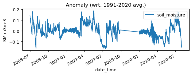
These 2 adapters are used to transform absolute values into anomalies on-the-fly after reading. You can select one or multiple columns for which the anomalies are computed. Additional kwargs (like timespan) are passed to the underlying anomaly and climatology function. For more details there is a separate tutorial available.
[19]:
from pytesmo.validation_framework.adapters import AnomalyClimAdapter
ds_mask = AnomalyClimAdapter(ismn_reader, columns=['soil_moisture'],
                             timespan=(datetime(1991,1,1), datetime(2020,12,31)))
anom = ds_mask.read(ids[0])
pprint(anom)
anom.plot(title='Anomaly (wrt. 1991-2020 avg.)', ylabel='SM m3m-3', figsize=(7,2))
                     soil_moisture soil_moisture_flag soil_moisture_orig_flag
date_time
2008-07-01 00:00:00       0.140861                C03                       M
2008-07-01 01:00:00       0.140861                C03                       M
2008-07-01 02:00:00       0.140861                C03                       M
2008-07-01 03:00:00       0.140861                C03                       M
2008-07-01 04:00:00       0.140861                C03                       M
...                            ...                ...                     ...
2010-07-31 19:00:00      -0.151816                  U                       M
2010-07-31 20:00:00      -0.151816                  U                       M
2010-07-31 21:00:00      -0.151816                  U                       M
2010-07-31 22:00:00      -0.151816                  U                       M
2010-07-31 23:00:00      -0.151816                  U                       M

[15927 rows x 3 columns]
[19]:
<Axes: title={'center': 'Anomaly (wrt. 1991-2020 avg.)'}, xlabel='date_time', ylabel='SM m3m-3'>
ColumnCombineAdapter
This adapter is used to combine multiple columns of a dataset after reading the time series. It takes any function that can be applied accross multiple columns and will add a new column of the chosen name to the data frame. E.g. in the following example we combine the proc_flag and snow_prob and frozen_prob column into a new column good that is ‘True’ when all the chosen columns are 0 and otherwise ‘False’. Then we apply a SelfMaskingAdapter that uses the newly added column
to filter the dataset. This is just for demonstration, we could also just use the AdvancedMaskingAdapter for this example. A more common use case for the ColumnCombineAdapter would be to compute the average when multiple soil moisture fields are available in a dataset.
This example also shows that you can stack multiple adapters together. If they depend on each other, it is important to notice that the innermost adapter will be called first!
[20]:
from pytesmo.validation_framework.adapters import ColumnCombineAdapter, SelfMaskingAdapter

def select_good(x):
    return (x['proc_flag'] == 0) and (x['snow_prob'] == 0) and (x['frozen_prob'] == 0)

ds_mask = SelfMaskingAdapter(ColumnCombineAdapter(ascat_reader, func=select_good, new_name='good'),
                             '==', True, 'good')
pprint(ds_mask.read(1814367)[['sm', 'proc_flag', 'snow_prob', 'frozen_prob', 'good']])
                              sm  proc_flag  snow_prob  frozen_prob  good
2007-06-03 03:33:38.999992  84.0          0          0            0  True
2007-06-03 14:51:50.999997  82.0          0          0            0  True
2007-06-06 02:31:33.000005  76.0          0          0            0  True
2007-06-06 13:49:46.999999  75.0          0          0            0  True
2007-06-08 03:30:13.000023  83.0          0          0            0  True
...                          ...        ...        ...          ...   ...
2014-06-25 13:51:37.000006  83.0          0          0            0  True
2014-06-27 03:32:04.999979  79.0          0          0            0  True
2014-06-27 14:50:18.000019  81.0          0          0            0  True
2014-06-30 02:30:05.000000  77.0          0          0            0  True
2014-06-30 13:48:17.999999  83.0          0          0            0  True

[713 rows x 5 columns]
[ ]: