Examples¶

Reading and plotting data from the ISMN¶

This example program chooses a random Network and Station and plots the first variable,depth,sensor combination. To see how to get data for a variable from all stations see the next example.

It can be found in the /examples folder of the pytesmo package under the name plot_ISMN_data.py.

In[1]:

import pytesmo.io.ismn.interface as ismn
import os
import matplotlib.pyplot as plt
import random

In[2]:

#path unzipped file downloaded from the ISMN web portal
#on windows the first string has to be your drive letter
#like 'C:\\'
path_to_ismn_data = os.path.join('D:\\','small_projects','cpa_2013_07_ISMN_userformat_reader',
                                      'header_values_parser_test')

In[3]:

#initialize interface, this can take up to a few minutes the first
#time, since all metadata has to be collected
ISMN_reader = ismn.ISMN_Interface(path_to_ismn_data)

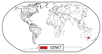
#plot available station on a map
fig, ax = ISMN_reader.plot_station_locations()
plt.show()

In[4]:

#select random network and station to plot
networks = ISMN_reader.list_networks()
print "Available Networks:"
print networks

Available Networks:
['OZNET']

In[5]:

network = random.choice(networks)
stations = ISMN_reader.list_stations(network = network)
print "Available Stations in Network %s"%network
print stations

Available Stations in Network OZNET
['Alabama' 'Balranald-Bolton_Park' 'Banandra' 'Benwerrin' 'Bundure'
 'Canberra_Airport' 'Cheverelis' 'Cooma_Airfield' 'Cootamundra_Aerodrome'
 'Cox' 'Crawford' 'Dry_Lake' 'Eulo' 'Evergreen' 'Ginninderra_K4'
 'Ginninderra_K5' 'Griffith_Aerodrome' 'Hay_AWS' 'Keenan' 'Kyeamba_Downs'
 'Kyeamba_Mouth' 'Kyeamba_Station' 'Rochedale' 'S_Coleambally' 'Samarra'
 'Silver_Springs' 'Spring_Bank' 'Strathvale' 'Uri_Park' 'Waitara'
 'Weeroona' 'West_Wyalong_Airfield' 'Widgiewa' 'Wollumbi' 'Wynella'
 'Yamma_Road' 'Yammacoona' 'Yanco_Research_Station']

In[6]:

station = random.choice(stations)
station_obj = ISMN_reader.get_station(station)
print "Available Variables at Station %s"%station
#get the variables that this station measures
variables = station_obj.get_variables()
print variables

Available Variables at Station Evergreen
['precipitation' 'soil moisture' 'soil temperature']

In[7]:

#to make sure the selected variable is not measured
#by different sensors at the same depths
#we also select the first depth and the first sensor
#even if there is only one
depths_from,depths_to = station_obj.get_depths(variables[0])

sensors = station_obj.get_sensors(variables[0],depths_from[0],depths_to[0])

#read the data of the variable, depth, sensor combination
time_series = station_obj.read_variable(variables[0],depth_from=depths_from[0],depth_to=depths_to[0],sensor=sensors[0])

#print information about the selected time series
print "Selected time series is:"
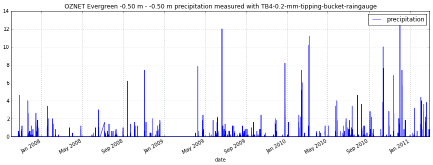
print time_series

Selected time series is:
OZNET Evergreen -0.50 m - -0.50 m precipitation measured with TB4-0.2-mm-tipping-bucket-raingauge

In[8]:

#plot the data
time_series.plot()
#with pandas 0.12 time_series.plot() also works
plt.legend()
plt.show()

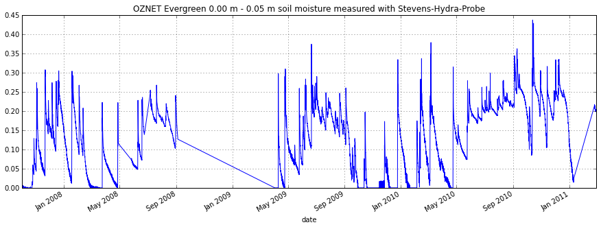
In[9]:

#we also want to see soil moisture
sm_depht_from,sm_depht_to = station_obj.get_depths('soil moisture')
print sm_depht_from,sm_depht_to

[ 0.   0.   0.3  0.6] [ 0.05  0.3   0.6   0.9 ]

In[10]:

#read sm data measured in first layer 0-0.05m
sm = station_obj.read_variable('soil moisture',depth_from=0,depth_to=0.05)
sm.plot()
plt.show()

Calculating anomalies and climatologies¶

This Example script reads and plots ASCAT H25 SSM data. The pytesmo.time_series.anomaly module is then used to calculate anomalies and climatologies of the time series. It can be found in the /examples folder of the pytesmo package under the name anomalies.py

import pytesmo.io.sat.ascat as ascat
import pytesmo.time_series as ts

import os
import matplotlib.pyplot as plt

ascat_folder = os.path.join('R:\\','Datapool_processed','WARP','WARP5.5',
                                         'ASCAT_WARP5.5_R1.2','080_ssm','netcdf')
ascat_grid_folder = os.path.join('R:\\','Datapool_processed','WARP','ancillary','warp5_grid')
#init the ASCAT_SSM reader with the paths

ascat_SSM_reader = ascat.AscatH25_SSM(ascat_folder,ascat_grid_folder)

ascat_ts = ascat_SSM_reader.read_ssm(45,0)
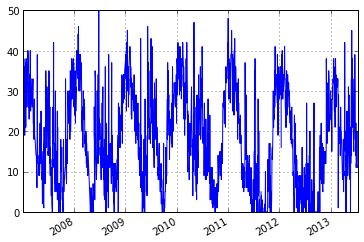
#plot soil moisture
ascat_ts.data['sm'].plot()

<matplotlib.axes.AxesSubplot at 0x22ee3550>

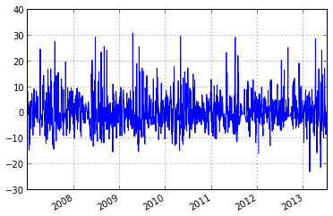
#calculate anomaly based on moving +- 17 day window
anomaly = ts.anomaly.calc_anomaly(ascat_ts.data['sm'], window_size=35)
anomaly.plot()

<matplotlib.axes.AxesSubplot at 0x269109e8>

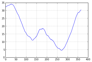
#calculate climatology
climatology = ts.anomaly.calc_climatology(ascat_ts.data['sm'])
climatology.plot()

<matplotlib.axes.AxesSubplot at 0x1bc54ef0>

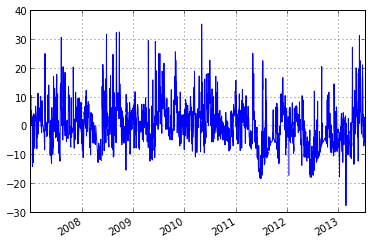
#calculate anomaly based on climatology
anomaly_clim = ts.anomaly.calc_anomaly(ascat_ts.data['sm'], climatology=climatology)
anomaly_clim.plot()

<matplotlib.axes.AxesSubplot at 0x1bc76860>

Calculation of the Soil Water Index¶

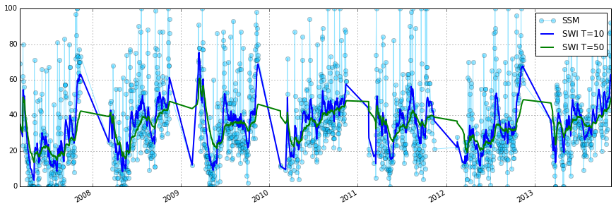
The Soil Water Index(SWI) which is a method to estimate root zone soil moisture can be calculated from Surface Soil Moisture(SSM) using an exponential Filter. For more details see this publication of C.Abergel et.al. The following example shows how to calculate the SWI for two T values from ASCAT H25 SSM.

import os

import matplotlib.pyplot as plt

from pytesmo.time_series.filters import exp_filter
import ascat


ascat_folder = os.path.join('/media', 'sf_R', 'Datapool_processed',
                            'WARP', 'WARP5.5', 'IRMA0_WARP5.5_P2',
                            'R1', '080_ssm', 'netcdf')
ascat_grid_folder = os.path.join('/media', 'sf_R',
                                 'Datapool_processed', 'WARP',
                                 'ancillary', 'warp5_grid')

# init the ASCAT_SSM reader with the paths

# ascat_folder is the path in which the cell files are
# located e.g. TUW_METOP_ASCAT_WARP55R12_0600.nc
# ascat_grid_folder is the path in which the file
# TUW_WARP5_grid_info_2_1.nc is located

# let's not include the orbit direction since it is saved as 'A'
# or 'D' it can not be plotted

# the AscatH25_SSM class automatically detects the version of data
# that you have in your ascat_folder. Please do not mix files of
# different versions in one folder

ascat_SSM_reader = ascat.AscatH25_SSM(ascat_folder, ascat_grid_folder,
                                      include_in_df=['sm', 'sm_noise',
                                                     'ssf', 'proc_flag'])

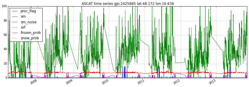
ascat_ts = ascat_SSM_reader.read_ssm(gpi, mask_ssf=True, mask_frozen_prob=10,
                                     mask_snow_prob=10)
ascat_ts.plot()

# Drop NA measurements
ascat_sm_ts = ascat_ts.data[['sm', 'sm_noise']].dropna()

# Get julian dates of time series
jd = ascat_sm_ts.index.to_julian_date().get_values()

# Calculate SWI T=10
ascat_sm_ts['swi_t10'] = exp_filter(ascat_sm_ts['sm'].values, jd, ctime=10)
ascat_sm_ts['swi_t50'] = exp_filter(ascat_sm_ts['sm'].values, jd, ctime=50)

fig, ax = plt.subplots(1, 1, figsize=(15, 5))
ascat_sm_ts['sm'].plot(ax=ax, alpha=0.4, marker='o',color='#00bfff', label='SSM')
ascat_sm_ts['swi_t10'].plot(ax=ax, lw=2,label='SWI T=10')
ascat_sm_ts['swi_t50'].plot(ax=ax, lw=2,label='SWI T=50')
plt.legend()

The pytesmo validation framework¶

The pytesmo validation framework takes care of iterating over datasets, spatial and temporal matching as well as sclaing. It uses metric calculators to then calculate metrics that are returned to the user. There are several metrics calculators included in pytesmo but new ones can be added simply by writing a new class.

Overview¶

How does the validation framework work? It makes these assumptions about the used datasets:

The dataset readers that are used have a read_ts method that can be called either by a grid point index (gpi) which can be any indicator that identifies a certain grid point or by using longitude and latitude. This means that both call signatures read_ts(gpi) and read_ts(lon, lat) must be valid. Please check the pygeobase documentation for more details on how a fully compatible dataset class should look. But a simple read_ts method should do for the validation framework. This assumption can be relaxed by using the read_ts_names keyword in the pytesmo.validation_framework.data_manager.DataManager class.
The read_ts method returns a pandas.DataFrame time series.
Ideally the datasets classes also have a grid attribute that is a pygeogrids grid. This makes the calculation of lookup tables easily possible and the nearest neighbor search faster.

Fortunately these assumptions are true about the dataset readers included in pytesmo.

It also makes a few assumptions about how to perform a validation. For a comparison study it is often necessary to choose a spatial reference grid, a temporal reference and a scaling or data space reference.

Spatial reference¶

The spatial reference is the one to which all the other datasets are matched spatially. Often through nearest neighbor search. The validation framework uses grid points of the dataset specified as the spatial reference to spatially match all the other datasets with nearest neighbor search. Other, more sophisticated spatial matching algorithms are not implemented at the moment. If you need a more complex spatial matching then a preprocessing of the data is the only option at the moment.

Temporal reference¶

The temporal reference is the dataset to which the other dataset are temporally matched. That means that the nearest observation to the reference timestamps in a certain time window is chosen for each comparison dataset. This is by default done by the temporal matching module included in pytesmo. How many datasets should be matched to the reference dataset at once can be configured, we will cover how to do this later.

Data space reference¶

It is often necessary to bring all the datasets into a common data space by using scaling. Pytesmo offers a choice of several scaling algorithms (e.g. CDF matching, min-max scaling, mean-std scaling, triple collocation based scaling). The data space reference can also be chosen independently from the other two references. New scaling methods can be implemented by writing a scaler class. An example of a scaler class can be found in the pytesmo.validation_framework.data_scalers.DefaultScaler.

Data Flow¶

After it is initialized, the validation framework works through the following steps:

Read all the datasets for a certain job (gpi, lon, lat)
Read all the masking datasets if any
Mask the temporal reference dataset using the masking data
Temporally match all the chosen combinations of temporal reference and other datasets
Scale all datasets into the data space of the data space reference, if scaling is activated
Turn the temporally matched time series over to the metric calculators
Get the calculated metrics from the metric calculators
Put all the metrics into a dictionary by dataset combination and return them.

Masking datasets¶

Masking datasets can be used if the the datasets that are compared do not contain the necessary information to mask them. For example we might want to use modelled soil temperature data to mask our soil moisture observations before comparing them. To be able to do that we just need a Dataset that returns a pandas.DataFrame with one column of boolean data type. Everywhere where the masking dataset is True the data will be masked.

Let’s look at a first example.

Example soil moisture validation: ASCAT - ISMN¶

This example shows how to setup the pytesmo validation framework to perform a comparison between ASCAT and ISMN data.

import os
import tempfile

import pytesmo.validation_framework.metric_calculators as metrics_calculators

from datetime import datetime

from ascat.timeseries import AscatSsmCdr
from pytesmo.io.ismn.interface import ISMN_Interface
from pytesmo.validation_framework.validation import Validation
from pytesmo.validation_framework.results_manager import netcdf_results_manager

First we initialize the data readers that we want to use. In this case the ASCAT soil moisture time series and in situ data from the ISMN.

Initialize ASCAT reader

ascat_data_folder = os.path.join('/home', 'cpa', 'workspace', 'pytesmo',
                                 'tests', 'test-data', 'sat', 'ascat', 'netcdf', '55R22')
ascat_grid_folder = os.path.join('/media/sf_R', 'Datapool_processed', 'WARP',
                                 'ancillary', 'warp5_grid')
static_layers_folder = os.path.join('/home', 'cpa', 'workspace', 'pytesmo',
                                    'tests', 'test-data', 'sat',
                                    'h_saf', 'static_layer')


ascat_reader = AscatSsmCdr(ascat_data_folder, ascat_grid_folder,
                           static_layer_path=static_layers_folder)

Initialize ISMN reader

ismn_data_folder = '/data/Development/python/workspace/pytesmo/tests/test-data/ismn/multinetwork/header_values/'
ismn_reader = ISMN_Interface(ismn_data_folder)

The validation is run based on jobs. A job consists of at least three lists or numpy arrays specifing the grid point index, its latitude and longitude. In the case of the ISMN we can use the dataset_ids that identify every time series in the downloaded ISMN data as our grid point index. We can then get longitude and latitude from the metadata of the dataset.

DO NOT CHANGE the name *jobs* because it will be searched during the parallel processing!

jobs = []

ids = ismn_reader.get_dataset_ids(variable='soil moisture', min_depth=0, max_depth=0.1)
for idx in ids:
    metadata = ismn_reader.metadata[idx]
    jobs.append((idx, metadata['longitude'], metadata['latitude']))
print jobs

[(0, 102.13330000000001, 33.666600000000003), (1, 102.13330000000001, 33.883299999999998), (2, -120.9675, 38.430030000000002), (3, -120.78559, 38.149560000000001), (4, -120.80638999999999, 38.17353), (5, -105.417, 34.25), (6, -97.082999999999998, 37.133000000000003), (7, -86.549999999999997, 34.783000000000001)]

For this small test dataset it is only one job

It is important here that the ISMN reader has a read_ts function that works by just using the dataset_id. In this way the validation framework can go through the jobs and read the correct time series.

data = ismn_reader.read_ts(ids[0])
print data.head()

                     soil moisture soil moisture_flag soil moisture_orig_flag
date_time
2008-07-01 00:00:00           0.45                  U                       M
2008-07-01 01:00:00           0.45                  U                       M
2008-07-01 02:00:00           0.45                  U                       M
2008-07-01 03:00:00           0.45                  U                       M
2008-07-01 04:00:00           0.45                  U                       M

Initialize the Validation class¶

The Validation class is the heart of the validation framwork. It contains the information about which datasets to read using which arguments or keywords and if they are spatially compatible. It also contains the settings about which metric calculators to use and how to perform the scaling into the reference data space. It is initialized in the following way:

datasets = {'ISMN': {'class': ismn_reader,
                     'columns': ['soil moisture']},
            'ASCAT': {'class': ascat_reader, 'columns': ['sm'],
                      'kwargs': {'mask_frozen_prob': 80,
                                 'mask_snow_prob': 80,
                                 'mask_ssf': True}}
           }

The datasets dictionary contains all the information about the datasets to read. The class is the dataset class to use which we have already initialized. The columns key describes which columns of the dataset interest us for validation. This a mandatory field telling the framework which other columns to ignore. In this case the columns soil moisture_flag and soil moisture_orig_flag will be ignored by the ISMN reader. We can also specify additional keywords that should be given to the read_ts method of the dataset reader. In this case we want the ASCAT reader to mask the ASCAT soil moisture using the included frozen and snow probabilities as well as the SSF. There are also other keys that can be used here. Please see the documentation for explanations.

period = [datetime(2007, 1, 1), datetime(2014, 12, 31)]
basic_metrics = metrics_calculators.BasicMetrics(other_name='k1')

process = Validation(
    datasets, 'ISMN', {(2, 2): basic_metrics.calc_metrics},
    temporal_ref='ASCAT',
    scaling='lin_cdf_match',
    scaling_ref='ASCAT',
    period=period)

During the initialization of the Validation class we can also tell it other things that it needs to know. In this case it uses the datasets we have specified earlier. The spatial reference is the 'ISMN' dataset which is the second argument. The third argument looks a little bit strange so let’s look at it in more detail.

It is a dictionary with a tuple as the key and a function as the value. The key tuple (n, k) has the following meaning: n datasets are temporally matched together and then given in sets of k columns to the metric calculator. The metric calculator then gets a DataFrame with the columns [‘ref’, ‘k1’, ‘k2’ …] and so on depending on the value of k. The value of (2, 2) makes sense here since we only have two datasets and all our metrics also take two inputs.

This can be used in more complex scenarios to e.g. have three input datasets that are all temporally matched together and then combinations of two input datasets are given to one metric calculator while all three datasets are given to another metric calculator. This could look like this:

{ (3 ,2): metric_calc,
  (3, 3): triple_collocation}

Create the variable *save_path* which is a string representing the path where the results will be saved. DO NOT CHANGE the name *save_path* because it will be searched during the parallel processing!

save_path = tempfile.mkdtemp()

import pprint
for job in jobs:

    results = process.calc(*job)
    pprint.pprint(results)
    netcdf_results_manager(results, save_path)

{(('ASCAT', 'sm'), ('ISMN', 'soil moisture')): {'BIAS': array([-0.04330891], dtype=float32),
                                                'R': array([ 0.7128256], dtype=float32),
                                                'RMSD': array([ 7.72966719], dtype=float32),
                                                'gpi': array([0], dtype=int32),
                                                'lat': array([ 33.6666]),
                                                'lon': array([ 102.1333]),
                                                'n_obs': array([384], dtype=int32),
                                                'p_R': array([ 0.], dtype=float32),
                                                'p_rho': array([ 0.], dtype=float32),
                                                'p_tau': array([ nan], dtype=float32),
                                                'rho': array([ 0.70022893], dtype=float32),
                                                'tau': array([ nan], dtype=float32)}}
{(('ASCAT', 'sm'), ('ISMN', 'soil moisture')): {'BIAS': array([ 0.237454], dtype=float32),
                                                'R': array([ 0.4996146], dtype=float32),
                                                'RMSD': array([ 11.58347607], dtype=float32),
                                                'gpi': array([1], dtype=int32),
                                                'lat': array([ 33.8833]),
                                                'lon': array([ 102.1333]),
                                                'n_obs': array([357], dtype=int32),
                                                'p_R': array([  6.12721281e-24], dtype=float32),
                                                'p_rho': array([  2.47165110e-28], dtype=float32),
                                                'p_tau': array([ nan], dtype=float32),
                                                'rho': array([ 0.53934574], dtype=float32),
                                                'tau': array([ nan], dtype=float32)}}
{(('ASCAT', 'sm'), ('ISMN', 'soil moisture')): {'BIAS': array([-0.63301021], dtype=float32),
                                                'R': array([ 0.78071409], dtype=float32),
                                                'RMSD': array([ 14.57700157], dtype=float32),
                                                'gpi': array([2], dtype=int32),
                                                'lat': array([ 38.43003]),
                                                'lon': array([-120.9675]),
                                                'n_obs': array([482], dtype=int32),
                                                'p_R': array([ 0.], dtype=float32),
                                                'p_rho': array([ 0.], dtype=float32),
                                                'p_tau': array([ nan], dtype=float32),
                                                'rho': array([ 0.69356072], dtype=float32),
                                                'tau': array([ nan], dtype=float32)}}
{(('ASCAT', 'sm'), ('ISMN', 'soil moisture')): {'BIAS': array([-1.9682411], dtype=float32),
                                                'R': array([ 0.79960084], dtype=float32),
                                                'RMSD': array([ 13.06224251], dtype=float32),
                                                'gpi': array([3], dtype=int32),
                                                'lat': array([ 38.14956]),
                                                'lon': array([-120.78559]),
                                                'n_obs': array([141], dtype=int32),
                                                'p_R': array([  1.38538225e-32], dtype=float32),
                                                'p_rho': array([  4.62621032e-39], dtype=float32),
                                                'p_tau': array([ nan], dtype=float32),
                                                'rho': array([ 0.84189808], dtype=float32),
                                                'tau': array([ nan], dtype=float32)}}
{(('ASCAT', 'sm'), ('ISMN', 'soil moisture')): {'BIAS': array([-0.21823417], dtype=float32),
                                                'R': array([ 0.80635566], dtype=float32),
                                                'RMSD': array([ 12.90389824], dtype=float32),
                                                'gpi': array([4], dtype=int32),
                                                'lat': array([ 38.17353]),
                                                'lon': array([-120.80639]),
                                                'n_obs': array([251], dtype=int32),
                                                'p_R': array([ 0.], dtype=float32),
                                                'p_rho': array([  4.20389539e-45], dtype=float32),
                                                'p_tau': array([ nan], dtype=float32),
                                                'rho': array([ 0.74206454], dtype=float32),
                                                'tau': array([ nan], dtype=float32)}}
{(('ASCAT', 'sm'), ('ISMN', 'soil moisture')): {'BIAS': array([-0.14228749], dtype=float32),
                                                'R': array([ 0.50703788], dtype=float32),
                                                'RMSD': array([ 14.24668026], dtype=float32),
                                                'gpi': array([5], dtype=int32),
                                                'lat': array([ 34.25]),
                                                'lon': array([-105.417]),
                                                'n_obs': array([1927], dtype=int32),
                                                'p_R': array([ 0.], dtype=float32),
                                                'p_rho': array([  3.32948515e-42], dtype=float32),
                                                'p_tau': array([ nan], dtype=float32),
                                                'rho': array([ 0.30299741], dtype=float32),
                                                'tau': array([ nan], dtype=float32)}}
{(('ASCAT', 'sm'), ('ISMN', 'soil moisture')): {'BIAS': array([ 0.2600247], dtype=float32),
                                                'R': array([ 0.53643185], dtype=float32),
                                                'RMSD': array([ 21.19682884], dtype=float32),
                                                'gpi': array([6], dtype=int32),
                                                'lat': array([ 37.133]),
                                                'lon': array([-97.083]),
                                                'n_obs': array([1887], dtype=int32),
                                                'p_R': array([ 0.], dtype=float32),
                                                'p_rho': array([ 0.], dtype=float32),
                                                'p_tau': array([ nan], dtype=float32),
                                                'rho': array([ 0.53143877], dtype=float32),
                                                'tau': array([ nan], dtype=float32)}}
{(('ASCAT', 'sm'), ('ISMN', 'soil moisture')): {'BIAS': array([-0.04437888], dtype=float32),
                                                'R': array([ 0.6058206], dtype=float32),
                                                'RMSD': array([ 17.3883934], dtype=float32),
                                                'gpi': array([7], dtype=int32),
                                                'lat': array([ 34.783]),
                                                'lon': array([-86.55]),
                                                'n_obs': array([1652], dtype=int32),
                                                'p_R': array([ 0.], dtype=float32),
                                                'p_rho': array([ 0.], dtype=float32),
                                                'p_tau': array([ nan], dtype=float32),
                                                'rho': array([ 0.62204134], dtype=float32),
                                                'tau': array([ nan], dtype=float32)}}

The validation is then performed by looping over all the defined jobs and storing the results. You can see that the results are a dictionary where the key is a tuple defining the exact combination of datasets and columns that were used for the calculation of the metrics. The metrics itself are a dictionary of metric-name: numpy.ndarray which also include information about the gpi, lon and lat. Since all the information contained in the job is given to the metric calculator they can be stored in the results.

Storing of the results to disk is at the moment supported by the netcdf_results_manager which creates a netCDF file for each dataset combination and stores each metric as a variable. We can inspect the stored netCDF file which is named after the dictionary key:

import netCDF4
results_fname = os.path.join(save_path, 'ASCAT.sm_with_ISMN.soil moisture.nc')

with netCDF4.Dataset(results_fname) as ds:
    for var in ds.variables:
        print var, ds.variables[var][:]

n_obs [ 384  357  482  141  251 1927 1887 1652]
tau [ nan  nan  nan  nan  nan  nan  nan  nan]
gpi [0 1 2 3 4 5 6 7]
RMSD [  7.72966719  11.58347607  14.57700157  13.06224251  12.90389824
  14.24668026  21.19682884  17.3883934 ]
lon [ 102.1333   102.1333  -120.9675  -120.78559 -120.80639 -105.417    -97.083
  -86.55   ]
p_tau [ nan  nan  nan  nan  nan  nan  nan  nan]
BIAS [-0.04330891  0.237454   -0.63301021 -1.9682411  -0.21823417 -0.14228749
  0.2600247  -0.04437888]
p_rho [  0.00000000e+00   2.47165110e-28   0.00000000e+00   4.62621032e-39
   4.20389539e-45   3.32948515e-42   0.00000000e+00   0.00000000e+00]
rho [ 0.70022893  0.53934574  0.69356072  0.84189808  0.74206454  0.30299741
  0.53143877  0.62204134]
lat [ 33.6666   33.8833   38.43003  38.14956  38.17353  34.25     37.133
  34.783  ]
R [ 0.7128256   0.4996146   0.78071409  0.79960084  0.80635566  0.50703788
  0.53643185  0.6058206 ]
p_R [  0.00000000e+00   6.12721281e-24   0.00000000e+00   1.38538225e-32
   0.00000000e+00   0.00000000e+00   0.00000000e+00   0.00000000e+00]

Parallel processing¶

The same code can be executed in parallel by defining the following start_processing function.

def start_processing(job):
    try:
        return process.calc(*job)
    except RuntimeError:
        return process.calc(*job)

pytesmo.validation_framework.start_validation can then be used to run your validation in parallel. Your setup code can look like this Ipython notebook without the loop over the jobs. Otherwise the validation would be done twice. Save it into a .py file e.g. my_validation.py.

After starting the ipyparallel cluster you can then execute the following code:

from pytesmo.validation_framework import start_validation

# Note that before starting the validation you must start a controller
# and engines, for example by using: ipcluster start -n 4
# This command will launch a controller and 4 engines on the local machine.
# Also, do not forget to change the setup_code path to your current setup.

setup_code = "my_validation.py"
start_validation(setup_code)

Masking datasets¶

Masking datasets are datasets that return a pandas DataFrame with boolean values. True means that the observation should be masked, False means it should be kept. All masking datasets are temporally matched in pairs to the temporal reference dataset. Only observations for which all masking datasets have a value of False are kept for further validation.

The masking datasets have the same format as the dataset dictionary and can be specified in the Validation class with the masking_datasets keyword.

Masking adapter¶

To easily transform an existing dataset into a masking dataset pytesmo offers a adapter class that calls the read_ts method of an existing dataset and performs the masking based on an operator and a given threshold.

from pytesmo.validation_framework.adapters import MaskingAdapter

ds_mask = MaskingAdapter(ismn_reader, '<', 0.2)
print ds_mask.read_ts(ids[0])['soil moisture'].head()

date_time
2008-07-01 00:00:00    False
2008-07-01 01:00:00    False
2008-07-01 02:00:00    False
2008-07-01 03:00:00    False
2008-07-01 04:00:00    False
Name: soil moisture, dtype: bool

Triple collocation and triple collocation based scaling¶

This example shows how to use the triple collocation routines in the pytesmo.metrics module. It also is a crash course to the theory behind triple collocation and links to relevant publications.

Triple collocation¶

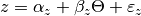
Triple collocation can be used to estimate the random error variance in three collocated datasets of the same geophysical variable [Stoffelen_1998]. Triple collocation assumes the following error model for each time series:

$X = \alpha + \beta\Theta + \varepsilon$

in which $\Theta$ is the true value of the geophysical variable e.g. soil moisture. $\alpha$ and $\beta$ are additive and multiplicative biases of the data and $\varepsilon$ is a zero mean random noise which we want to estimate.

Estimation of the triple collocation error $\varepsilon$ is commonly done using one of two approaches:

Scaling/calibrating the datasets to a reference dataset (removing $\alpha$ and $\beta$ ) and calculating the triple collocation error based on these datasets.
Estimation of the triple collocation error based on the covariances between the datasets. This also yields (linear) scaling parameters ( $\beta$ ) which can be used if scaling of the datasets is desired.

Note

The scaling approaches commonly used in approach 1 are not ideal for e.g. data assimilation. Under the assumption that assimilated observations should have orthogonal errors, triple collocation based scaling parameters are ideal [Yilmaz_2013].

Approach 2 is recommended for scaling if three datasets are available.

Generate a synthetic dataset¶

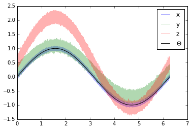
We can now make three synthetic time series based on the defined error model:

$x = \alpha_x + \beta_x\Theta + \varepsilon_x$

$y = \alpha_y + \beta_y\Theta + \varepsilon_y$

$z = \alpha_z + \beta_z\Theta + \varepsilon_z$

In which we will assume that our $\Theta$ i.e. the real observed signal, is a simple sine curve.

import numpy as np
import matplotlib.pyplot as plt

# number of observations
n = 1000000
# x coordinates for initializing the sine curve
coord = np.linspace(0, 2*np.pi, n)
signal = np.sin(coord)

# error i.e. epsilon of the three synthetic time series
sig_err_x = 0.02
sig_err_y = 0.07
sig_err_z = 0.04
err_x = np.random.normal(0, sig_err_x, n)
err_y = np.random.normal(0, sig_err_y, n)
err_z = np.random.normal(0, sig_err_z, n)

# additive and multiplicative biases
# they are assumed to be zero for dataset x
alpha_y = 0.2
alpha_z = 0.5

beta_y = 0.9
beta_z = 1.6

x = signal + err_x
# here we assume errors that are already scaled
y = alpha_y + beta_y * (signal + err_y)
z = alpha_z + beta_z * (signal + err_z)

plt.plot(coord, x, alpha=0.3, label='x')
plt.plot(coord, y, alpha=0.3, label='y')
plt.plot(coord, z, alpha=0.3, label='z')
plt.plot(coord, signal, 'k', label='$\Theta$')
plt.legend()
plt.show()

Approach 1¶

We can now use these three time series and estimate the $\varepsilon$ values using approach 1.

The functions we can be found in:

We will use mean-standard deviation scaling. This type of scaling brings the data to the same mean and standard deviation as the reference dataset.

import pytesmo.scaling as scaling
import pytesmo.metrics as metrics

# scale to x as the reference
y_scaled = scaling.mean_std(y, x)
z_scaled = scaling.mean_std(z, x)
plt.plot(coord, x, alpha=0.3, label='x')
plt.plot(coord, y_scaled, alpha=0.3, label='y scaled')
plt.plot(coord, z_scaled, alpha=0.3, label='z scaled')
plt.plot(coord, signal, 'k', label='$\Theta$')
plt.legend()
plt.show()

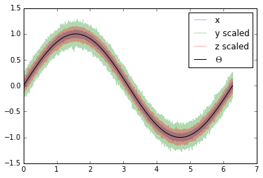
The three datasets do now have the same mean and standard deviation. This means that $\alpha$ and $\beta$ have been removed from $y$ and $z$ .

From these three scaled datasets we can now estimate the triple collocation error following the method outlined in [Scipal_2008]:

The basic formula (formula 4 in the paper) adapted to the notation we use in this tutorial is:

$\sigma_{\varepsilon_x}^2 = \langle (x-y_{scaled})(x-z_{scaled}) \rangle$

$\sigma_{\varepsilon_y}^2 = \langle (y_{scaled}-x)(y_{scaled}-z_{scaled}) \rangle$

$\sigma_{\varepsilon_z}^2 = \langle (z_{scaled}-x)(z_{scaled}-y_{scaled}) \rangle$

where the $\langle\rangle$ brackets mean the temporal mean. This function is implemented in pytesmo.metrics.tcol_error() which we can now use to estimate the standard deviation of $\varepsilon$ : $\sigma_{\varepsilon_i}$

e_x, e_y, e_z = metrics.tcol_error(x, y_scaled, z_scaled)
print "Error of x estimated: {:.4f}, true: {:.4f}".format(e_x, sig_err_x)
print "Error of y estimated: {:.4f}, true: {:.4f}".format(e_y, sig_err_y)
print "Error of z estimated: {:.4f}, true: {:.4f}".format(e_z, sig_err_z)

Error of x estimated: 0.0200, true: 0.0200
Error of y estimated: 0.0697, true: 0.0700
Error of z estimated: 0.0399, true: 0.0400

We can see that the estimated error standard deviation is very close to the one we set for our artificial time series in the beginning.

Approach 2¶

In approach 2 we can estimate the triple collocation errors, the scaling parameter $\beta$ and the signal to noise ratio directly from the covariances of the dataset. For a general overview and how approach 1 and 2 are related please see [Gruber_2015].

Estimation of the error variances from the covariances of the datasets (e.g. $\sigma_{XY}$ for the covariance between $x$ and $y$ ) is done using the following formula:

$\\\sigma_{\varepsilon_x}^2 = \sigma_{X}^2 - \frac{\sigma_{XY}\sigma_{XZ}}{\sigma_{YZ}}\\ \sigma_{\varepsilon_y}^2 = \sigma_{Y}^2 - \frac{\sigma_{YX}\sigma_{YZ}}{\sigma_{XZ}}\\ \sigma_{\varepsilon_z}^2 = \sigma_{Z}^2 - \frac{\sigma_{ZY}\sigma_{ZX}}{\sigma_{YX}}$

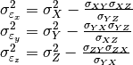
$\beta$ can also be estimated from the covariances:

$\beta_x = 1 \quad \quad \quad \beta_y = \frac{\sigma_{XZ}}{\sigma_{YZ}} \quad \quad \quad \beta_z=\frac{\sigma_{XY}}{\sigma_{ZY}}$

The signal to noise ratio (SNR) is also calculated from the variances and covariances:

$\\\text{SNR}_X[dB] = -10\log\left(\frac{\sigma_{X}^2\sigma_{YZ}}{\sigma_{XY}\sigma_{XZ}}-1\right)\\ \text{SNR}_Y[dB] = -10\log\left(\frac{\sigma_{Y}^2\sigma_{XZ}}{\sigma_{YX}\sigma_{YZ}}-1\right)\\ \text{SNR}_Z[dB] = -10\log\left(\frac{\sigma_{Z}^2\sigma_{XY}}{\sigma_{ZX}\sigma_{ZY}}-1\right)$

It is given in dB to make it symmetric around zero. If the value is zero it means that the signal variance and the noise variance are equal. +3dB means that the signal variance is twice as high as the noise variance.

This approach is implemented in pytesmo.metrics.tcol_snr().

snr, err, beta = metrics.tcol_snr(x, y, z)
print "Error of x approach 1: {:.4f}, approach 2: {:.4f}, true: {:.4f}".format(e_x, err[0], sig_err_x)
print "Error of y approach 1: {:.4f}, approach 2: {:.4f}, true: {:.4f}".format(e_y, err[1], sig_err_y)
print "Error of z approach 1: {:.4f}, approach 2: {:.4f}, true: {:.4f}".format(e_z, err[2], sig_err_z)

Error of x approach 1: 0.0200, approach 2: 0.0199, true: 0.0200
Error of y approach 1: 0.0697, approach 2: 0.0700, true: 0.0700
Error of z approach 1: 0.0399, approach 2: 0.0400, true: 0.0400

It can be seen that both approaches estimate very similar error variance.

We can now also check if $\beta_y$ and $\beta_z$ were correctly estimated.

The function gives us the inverse values of $\beta$ . We can use these values directly to scale our datasets.

print "scaling parameter for y estimated: {:.2f}, true:{:.2f}".format(1/beta[1], beta_y)
print "scaling parameter for z estimated: {:.2f}, true:{:.2f}".format(1/beta[2], beta_z)

scaling parameter for y estimated: 0.90, true:0.90
scaling parameter for z estimated: 1.60, true:1.60

y_beta_scaled = y * beta[1]
z_beta_scaled = z * beta[2]
plt.plot(coord, x, alpha=0.3, label='x')
plt.plot(coord, y_beta_scaled, alpha=0.3, label='y beta scaled')
plt.plot(coord, z_beta_scaled, alpha=0.3, label='z beta scaled')
plt.plot(coord, signal, 'k', label='$\Theta$')
plt.legend()
plt.show()

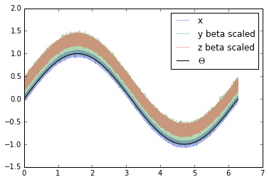
The datasets still have different mean values i.e. different $\alpha$ values. $\alpha$ can be estimated through the mean of the dataset.

y_ab_scaled = y_beta_scaled - np.mean(y_beta_scaled)
z_ab_scaled = z_beta_scaled - np.mean(z_beta_scaled)
plt.plot(coord, x, alpha=0.3, label='x')
plt.plot(coord, y_ab_scaled, alpha=0.3, label='y ab scaled')
plt.plot(coord, z_ab_scaled, alpha=0.3, label='z ab scaled')
plt.plot(coord, signal, 'k', label='$\Theta$')
plt.legend()
plt.show()

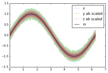
This yields scaled/calibrated datasets using triple collocation based scaling which is ideal for e.g. data assimilation.

The SNR is nothing else than the fraction of the signal variance to the noise variance in dB

Let’s first print the snr we got from pytesmo.metrics.tcol_snr()

print snr

[ 31.01493632  20.0865377   24.94339476]

Now let’s calculate the SNR starting from the variance of the sine signal and the $\sigma$ values we used for our additive errors.

[10*np.log10(np.var(signal)/(sig_err_x)**2),
10*np.log10(np.var(signal)/(sig_err_y)**2),
10*np.log10(np.var(signal)/(sig_err_z)**2)]

[30.969095787133575, 20.087734900128062, 24.94849587385395]

We can see that the estimated SNR and the “real” SNR of our artificial datasets are very similar.

References¶

[Stoffelen_1998]

Stoffelen, A. (1998). Toward the true near-surface wind speed: error modeling and calibration using triple collocation. Journal of Geophysical Research: Oceans (1978–2012), 103(C4), 7755–7766.

[Yilmaz_2013]

Yilmaz, M. T., & Crow, W. T. (2013). The optimality of potential rescaling approaches in land data assimilation. Journal of Hydrometeorology, 14(2), 650–660.

[Scipal_2008]

Scipal, K., Holmes, T., De Jeu, R., Naeimi, V., & Wagner, W. (2008). A possible solution for the problem of estimating the error structure of global soil moisture data sets. Geophysical Research Letters, 35(24), .

[Gruber_2015]

Gruber, A., Su, C., Zwieback, S., Crow, W., Dorigo, W., Wagner, W. (2015). Recent advances in (soil moisture) triple collocation analysis. International Journal of Applied Earth Observation and Geoinformation, in press. 10.1016/j.jag.2015.09.002

Comparing ASCAT and insitu data from the ISMN without the validation framework¶

This example program loops through all insitu stations that measure soil moisture with a depth between 0 and 0.1m it then finds the nearest ASCAT grid point and reads the ASCAT data. After temporal matching and scaling using linear CDF matching it computes several metrics, like the correlation coefficients(Pearson’s, Spearman’s and Kendall’s), Bias, RMSD as well as the Nash–Sutcliffe model efficiency coefficient.

It also shows the usage of the pytesmo.df_metrics module.

It is stopped after 2 stations to not take to long to run and produce a lot of plots

It can be found in the /examples folder of the pytesmo package under the name compare_ISMN_ASCAT.py.

import pytesmo.io.ismn.interface as ismn
import ascat
import pytesmo.temporal_matching as temp_match
import pytesmo.scaling as scaling
import pytesmo.df_metrics as df_metrics
import pytesmo.metrics as metrics

import os
import matplotlib.pyplot as plt

ascat_folder = os.path.join('R:\\','Datapool_processed','WARP','WARP5.5',
                                         'ASCAT_WARP5.5_R1.2','080_ssm','netcdf')
ascat_grid_folder = os.path.join('R:\\','Datapool_processed','WARP','ancillary','warp5_grid')
#init the ASCAT_SSM reader with the paths

#let's not include the orbit direction since it is saved as 'A'
#or 'D' it can not be plotted
ascat_SSM_reader = ascat.AscatH25_SSM(ascat_folder,ascat_grid_folder,
                                      include_in_df=['sm', 'sm_noise', 'ssf', 'proc_flag'])

#set path to ISMN data
path_to_ismn_data =os.path.join('D:\\','small_projects','cpa_2013_07_ISMN_userformat_reader','header_values_parser_test')
#Initialize reader
ISMN_reader = ismn.ISMN_Interface(path_to_ismn_data)

i = 0

label_ascat='sm'
label_insitu='insitu_sm'

#this loops through all stations that measure soil moisture
for station in ISMN_reader.stations_that_measure('soil moisture'):

    #this loops through all time series of this station that measure soil moisture
    #between 0 and 0.1 meters
    for ISMN_time_series in station.data_for_variable('soil moisture',min_depth=0,max_depth=0.1):

        ascat_time_series = ascat_SSM_reader.read_ssm(ISMN_time_series.longitude,
                                                      ISMN_time_series.latitude,
                                                      mask_ssf=True,
                                                      mask_frozen_prob = 5,
                                                      mask_snow_prob = 5)


        #drop nan values before doing any matching
        ascat_time_series.data = ascat_time_series.data.dropna()

        ISMN_time_series.data = ISMN_time_series.data.dropna()

        #rename the soil moisture column in ISMN_time_series.data to insitu_sm
        #to clearly differentiate the time series when they are plotted together
        ISMN_time_series.data.rename(columns={'soil moisture':label_insitu},inplace=True)

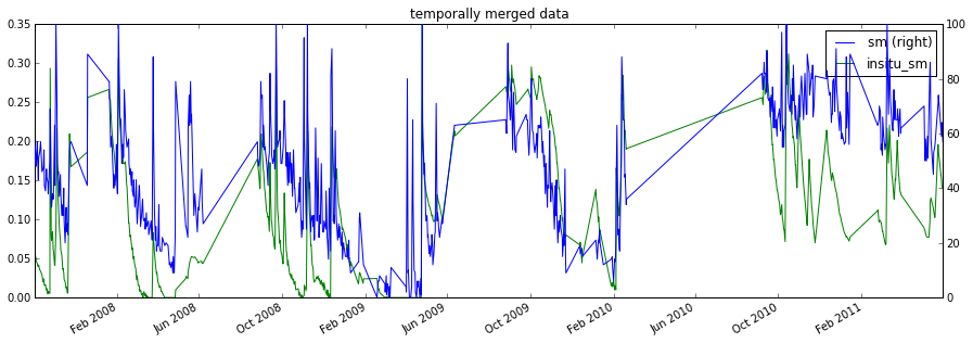
        #get ISMN data that was observerd within +- 1 hour(1/24. day) of the ASCAT observation
        #do not include those indexes where no observation was found
        matched_data = temp_match.matching(ascat_time_series.data,ISMN_time_series.data,
                                                window=1/24.)
        #matched ISMN data is now a dataframe with the same datetime index
        #as ascat_time_series.data and the nearest insitu observation

        #continue only with relevant columns
        matched_data = matched_data[[label_ascat,label_insitu]]

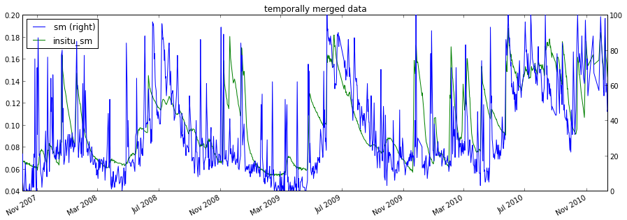
        #the plot shows that ISMN and ASCAT are observed in different units
        matched_data.plot(figsize=(15,5),secondary_y=[label_ascat],
                          title='temporally merged data')
        plt.show()

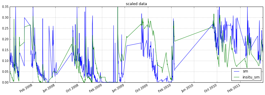
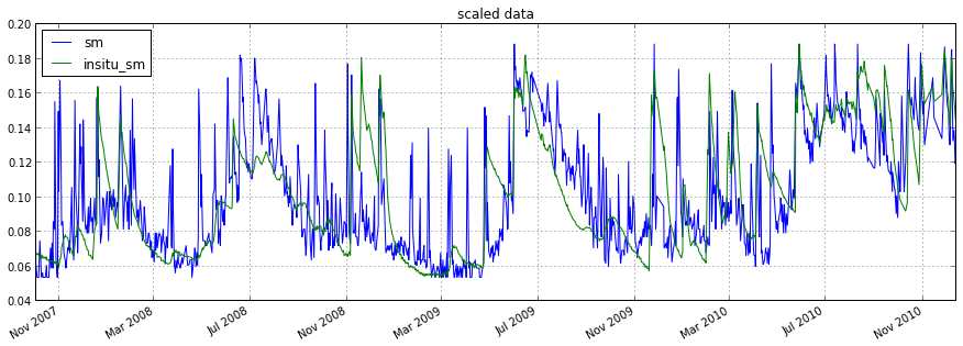
        #this takes the matched_data DataFrame and scales all columns to the
        #column with the given reference_index, in this case in situ
        scaled_data = scaling.scale(matched_data, method='lin_cdf_match',
                                         reference_index=1)

        #now the scaled ascat data and insitu_sm are in the same space
        scaled_data.plot(figsize=(15,5), title='scaled data')
        plt.show()

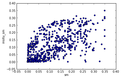
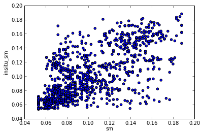
        plt.scatter(scaled_data[label_ascat].values,scaled_data[label_insitu].values)
        plt.xlabel(label_ascat)
        plt.ylabel(label_insitu)
        plt.show()

        #calculate correlation coefficients, RMSD, bias, Nash Sutcliffe
        x, y = scaled_data[label_ascat].values, scaled_data[label_insitu].values

        print "ISMN time series:",ISMN_time_series
        print "compared to"
        print ascat_time_series
        print "Results:"

        #df_metrics takes a DataFrame as input and automatically
        #calculates the metric on all combinations of columns
        #returns a named tuple for easy printing
        print df_metrics.pearsonr(scaled_data)
        print "Spearman's (rho,p_value)", metrics.spearmanr(x, y)
        print "Kendalls's (tau,p_value)", metrics.kendalltau(x, y)
        print df_metrics.kendalltau(scaled_data)
        print df_metrics.rmsd(scaled_data)
        print "Bias", metrics.bias(x, y)
        print "Nash Sutcliffe", metrics.nash_sutcliffe(x, y)


    i += 1

    #only show the first 2 stations, otherwise this program would run a long time
    #and produce a lot of plots
    if i >= 2:
        break

ISMN time series: OZNET Alabama 0.00 m - 0.05 m soil moisture measured with Stevens-Hydra-Probe
compared to
ASCAT time series gpi:1884359 lat:-35.342 lon:147.541
Results:
(Pearsons_r(sm_and_insitu_sm=0.61607679781575175), p_value(sm_and_insitu_sm=3.1170801211098453e-65))
Spearman's (rho,p_value) (0.64651747115098912, 1.0057610194056589e-73)
Kendalls's (tau,p_value) (0.4685441550995097, 2.4676437876515864e-67)
(Kendall_tau(sm_and_insitu_sm=0.4685441550995097), p_value(sm_and_insitu_sm=2.4676437876515864e-67))
rmsd(sm_and_insitu_sm=0.078018684719599857)
Bias 0.00168114697282
Nash Sutcliffe 0.246416864767

ISMN time series: OZNET Balranald-Bolton_Park 0.00 m - 0.08 m soil moisture measured with CS615
compared to
ASCAT time series gpi:1821003 lat:-33.990 lon:146.381
Results:
(Pearsons_r(sm_and_insitu_sm=0.66000287576696759), p_value(sm_and_insitu_sm=1.3332742454781072e-126))
Spearman's (rho,p_value) (0.65889275747696652, 4.890533231776912e-126)
Kendalls's (tau,p_value) (0.48653686844813893, 6.6517671082477896e-118)
(Kendall_tau(sm_and_insitu_sm=0.48653686844813893), p_value(sm_and_insitu_sm=6.6517671082477896e-118))
rmsd(sm_and_insitu_sm=0.028314835540753237)
Bias 4.56170862568e-05
Nash Sutcliffe 0.316925662899